Ēlýsion pedíon

You can read a Portuguese translation of this article here

In this article I’m showing an example of using mathematics in the real world. Every high school student has already seen the following electric circuit: 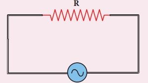It’s an alternate current circuit. In an electric circuit, we want to know all the currents and voltages on each electronic component. Knowing them, we can calculate all the powers generated(and absorbed) by each component. We can solve such circuits by using Kirchhoff’s Law and Ohm’s Law. It’s interesting to point out that for many students, this is the first physical example that they use complex numbers. To make things easy, we are going to assume the reader knows about Calculus.

Since solving such circuits is easy, we don’t need to waste time on it. When dealing with these problems in school, we have enough information to solve them. And, to make things easy, we always deal with systems of linear equations. But what happens when the student decides to solve an electrical network used in the real world, for example:

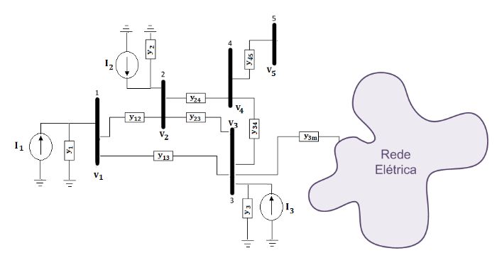
Not only is this circuit complex but we also don’t have enough information to solve it using Kirchhoff’s law directly, like the problem above. In mathematics, what we have here is more variables than equations. We can’t just assume some values for given variables since even if we can solve the system, it doesn’t mean it’s a valid solution(that is, it works for the real system). In other words, trying random values only solves the equation, but not the real world problem. Because of that, we need to find more equations to solve the system.

Each of the Buses above(1, 2, 3, etc) are defined by what we know about them. A $PV$ Bus, also called a Generator Bus, is so called because we know its active power and its voltage, and a $PQ$ Bus, also called Load Bus, is one we know both its active and reactive power. There is also a third type called a Swing/Slack bus(or $V\theta$ bus) that is used to check what are the power losses in the system. We can use Kirchhoff’s law to calculate the active and reactive power in each bus as a function of every other voltage, their angle, and also the admittance of the lines(that is, the physical properties of the transmission lines). Thus, we find the following equations:

$$P_{k}^{\text{calculated}} = V_{k}\Sigma_{m \in K}V_m (G_{km}\cos(\theta_{km}) + B_{km}\sin(\theta_{km}))\\ Q_{k}^{\text{calculated}} = V_{k}\Sigma_{m \in K}V_m (G_{km}\sin(\theta_{km}) - B_{km}\cos(\theta_{km}))$$

$K$ is the set of all buses in the system, $G$ and $B$ are the real and complex elements, respectively, of a matrix $Y$ called the bus admittance matrix. This matrix is created using the physical properties of the transmission lines. $G_{km}$ and $B_{km}$ are different from $0$ if and only if there is a connection between the buses $k$ and $m$. In most cases, there is no such connection and the matrix $Y$ has a lot of $0$. We call this kind of matrix a sparse matrix. $\theta$ is the angle of the voltage at a bus and $\theta_{km} = \theta_k - \theta_m$

As mentioned above, there are buses in which we know its active power and voltage($PV$) and which we know both active and reactive power($PQ$). With them, we can create equations for our system. For each bus we know its active power($PV$), we create the following equation:

$$P^{\text{known}}_k - P^{\text{calculated}}_k = 0$$

And for each bus we know both powers($PQ$), we have:

$$P^{\text{known}}_k - P^{\text{calculated}}_k = 0\\ Q^{\text{known}}_k - Q^{\text{calculated}}_k = 0$$

The objective is to know the state of the system in each bus, this means we know its voltage and angle of that voltage, since knowing them we can calculate its current(Ohm’s law gives us that, for $I = VY$, where $I$ is the current, $V$ is the voltage, and $Y$ is the admittance). We need to calculate the voltage’s angles because they are generated in an AC circuit and that can make both current and voltage not be in phase(which can affect the active power generated by the system) e thus we must know exactly the phase of the system. The buses we know the active and reactive power only tell us the values for $P_k$ and $Q_k$. but not for $V_k$ and $\theta_k$. Therefore, in the above equations, most of the $V_k$ and $\theta_k$ are variables we DON’T know its values, those we know are just constants in the equations. Those variables are exactly what we want to know. The number of equations we create depends on the number and types of buses we have. For each $PQ$ bus we have two equations and for each $PV$ we have one equations, se overall we have $2 * \#PQ + \#PV$ equations, where $\#PQ$ is the number of $PQ$ buses and $\#PV$ is the number of $PV$ buses. To make things worse, all the equations above are nonlinear.

Now that we have our system of equations, we just need to find the values for $V_k$ and $\theta_k$ such that the left side of the equations is $0$. In mathematics, this is the same as finding the values where the function vanishes. Methods to find the $0$ of a function, that is, a point $x_s$ where the function $g(x)$ has the value $g(x_s)=0$ are called “root-finding methods”. There are a lot of them and the one I’m going to mention, the one used a lot in this kind of problem, is called Newton-Raphson method. It’s also a great method to solve nonlinear systems of equations.

Let $g(x)$ be the following function: 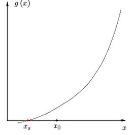We want to find the point $s$ such that $g(s)=0$. We take any point $x_0$ and calculate $g(x_0)$. If $x_0 = s$, great, but that rarely happens. Thus $g(x_0)$ is a point on the curve. Using the derivative, we can calculate the tangent line to the graph at the point $x_0$. With that, we can find out where the line touches the $x$-axis. This location is our point $x_1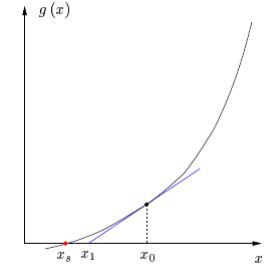$: We can repeat this process to approach the point $s$ little by little. The idea here is called an iterative method, where the method generates a point that we can use in the method again to generate a new point. In this way, we can approach a solution by using only the initial point and letting the method generate new points. The Newton-Raphson is an example of an iterative method.

The advantage of this method is that it generates a new point calculating both the tangent line and where it touches the $x$-axis. What it gives us is the distance between the old point and the new point, but given that $\Delta x = x_1 – x_0$, where $\Delta x$ is the distance between the points, we can calculate $x_1$ using $x_1 = x_0 + \Delta x$.

One can get the formula for the method by applying the Taylor series of the function and ignoring all the nonlinear terms. The formula is: $$\Delta x = -\frac{g(x)}{g'(x)}$$

It’s good to mention that the method rarely generates the exact solution, but only an approximation. An exact solution is not always possible, given that it could be a number such that its decimal representation has infinite, non repeating, numbers after the decimal point. But the method can always generate a good approximation, as good as we want. This is done by defining a very small positive value $\epsilon$, called the tolerance, such that $x$ is a solution if $|g(x)| \leq \epsilon $.

The following image shows the method being used to find a solution: 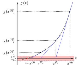We note that $x^{(3)}$ is a solution since $|g(x^{(3)})| \leq \epsilon$. Something that can happen is that the initial value doesn’t generate a solution(the tangent line can take the point further away from the solution, for example) and because of that we need to try another initial value. When we use a computer program to solve this problem, we take into account an iteration counter that finishes the method if after many iterations, no solution is found. This is an indication that the initial value is not a good point.

In the case of $M$ variables, which is our case here, the method is pretty much the same, the only difference is that instead of the derivative of the function, we have the Jacobian matrix, $\mathbf{J}$, which is a matrix formed by the partial derivatives of the function. In a system with $N$ equations and $M$ variables, we have a $N \times M$ matrix where for each equation(row) we have $M$ partial derivatives(columns). The method has the following formula: $$\Delta x = -\mathbf{J}(x)^{-1} \cdot g(x)$$ where $\mathbf{J}(x)^{-1}$ is the inverse of the Jacobian matrix.

In our case, $g(x)$ are the equations for the buses $PV$ and $PQ$ mentioned above. We take the jacobian matrix of this $g(x)$. The variables are $V_k$ and $\theta_k$. Our $\Delta x$ in this case is a column vector formed by $\Delta V_k$ and $\Delta \theta_k$. With this, we have all the tools to calculate the state of the system, our $V_k$ and $\theta_k$, in all buses.

So, that is it? In theory, yes. We can try different initial values and wait for the method to generate a solution. In a computer, this can be done without any problems (to be honest, there is a computational problem in generating the inverse of the Jacobian matrix, but we can ignore this here). But in the real world, this is not enough. I’m not going to enter in details, since here we find a lot of problems and also a lot of ways to solve this, including lots of simplifications we can use based on what we know about electric networks. But I’ll mention 2 important topics.

The first problem is that when a solution is generated some $Q_k$ may give wrong values. In a $PV$ bus, we know the values for the voltage at that bus and its active power, so we can try to calculate the reactive power generated(or absorbed) by that bus and find that the value of $Q$ is greater or less than pre-established limits $Q_{max}$ and $Q_{min}$. When this happens, it means that the voltage in that bus should change (increase or decrease depending on which limit $Q$ passed). Since in a $PV$, the voltage is specified, it can never change when new points are generated(that is, it doesn’t appear in the $\Delta V_k$ above), but since the value of $Q$ passed one of the limits, we expect the value of $V$ to change too. To work around this problem, we force the $PV$ bus to become a $PQ$ bus, taking the value for $Q$ one of the limits that $Q$ passed and forcing $V$ to become a variable of the system. This forces the system to add a new equation (the one for $Q$ in this bus). The Jacobian matrix gets a new column (the partial derivatives of each equation depending on V) and a new line (the partial derivatives of the new $Q$ equation). After doing this, we must check if the new values for $V$ are changing based on what we expect (increase or decrease based on the new value for $Q$) and if that happens, we keep the bus as a $PQ$ bus until we find a solution. In the case where the values for $V$ do not change as we expected, we have to go back to the case where the bus was a $PV$ bus. What this means is that as the method generates new points, it would fix the problem of the $Q$ not being between $Q_{max}$ and $Q_{min}$. One way of avoiding this useless change is to create a new tolerance $\sigma$ and only check if the value for $Q$ is valid after the method generate points such that $|g(x)| \leq \sigma$.

The second problem is for $PQ$ buses. In this case, what happens is that the value for $V$ may be greater or less than pre-established limits $V_{max}$ and $V_{min}$. In this case, we change a $PQ$ bus to a $PV$ bus. What was said above about going back or not can be repeated here.

Now, we have to ask something: why do we want to calculate all of this? Well, the answer is planning. Suppose we want to install new buses to transmit electricity to a new region. First, we need to check if the new buses are not going to bring us any new problems to the system or not. The method utilized above gives us a good idea where there are any problems, if the voltage drop in some bus is too much, if there are more than expected power losses, if the reactive power generated in some bus is affecting the system, etc. Applying this method, we can easily see if we can install new buses or if we need to do some changes in the existing system first.

And with this we have an example of using mathematics(and physics) in the real world.

#math